MLDL_정리/Sample
DL - Confusion Matrix
KimTory
2022. 2. 5. 01:15
Model 성능 평가 방법 - Confusion Matrix
→ 학습된 모델의 입력값과 예측값을 정리한 테이블을 Confusion Matrix 이라고 한다.
→ Confusion Matrix를 통해서 모델의 성능지표인 Accuracy, Precision, Recall, F1 Score를 계산
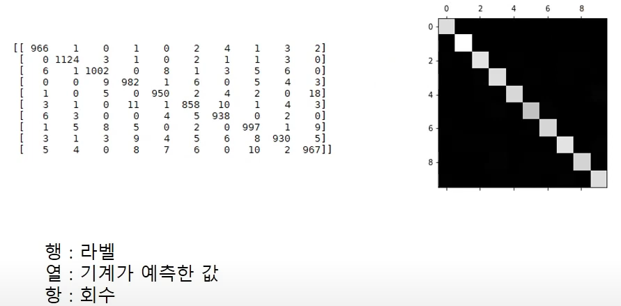
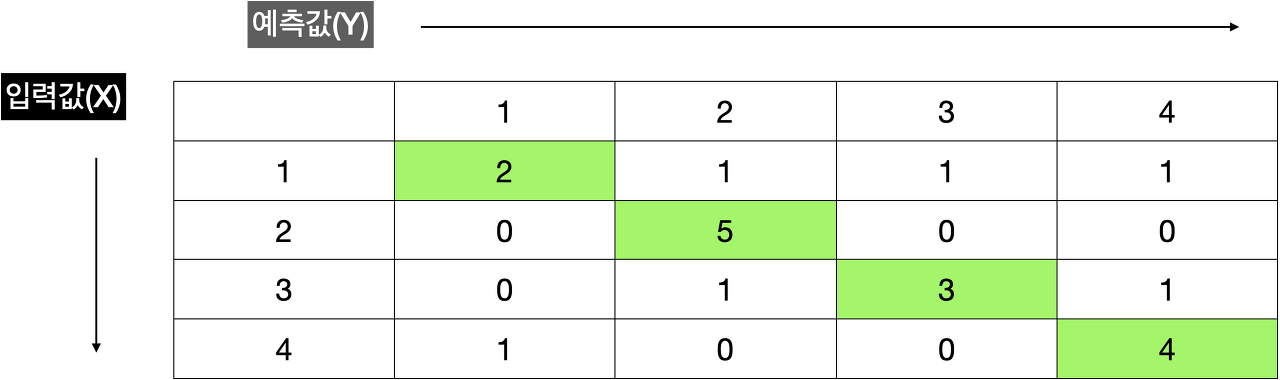
Confusion Matrix 보면 학습된 모델에게 '1'을 5번 보여줬을때 2번 맞췄다는걸 알 수 있습니다.
'2'는 5번, '3'은 3번 , '4'는 4번 맞춘걸 알 수 있습니다.
import sys, os
sys.path.append(os.pardir)

import numpy as np
from dataset.mnist import load_mnist
from two_layer_net import TwoLayerNet
import pickle

# 데이터 읽기
(x_train, t_train), (x_test, t_test) = load_mnist(normalize=True, one_hot_label=True)

network = TwoLayerNet(input_size=784, hidden_size=50, output_size=10)

iters_num = 10000
train_size = x_train.shape[0]
batch_size = 100
learning_rate = 0.1

train_loss_list = []
train_acc_list = []
test_acc_list = []

iter_per_epoch = max(train_size / batch_size, 1)

for i in range(iters_num):
    batch_mask = np.random.choice(train_size, batch_size)
    x_batch = x_train[batch_mask]
    t_batch = t_train[batch_mask]

    # 기울기 계산
    #grad = network.numerical_gradient(x_batch, t_batch) # 수치 미분 방식
    grad = network.gradient(x_batch, t_batch) # 오차역전파법 방식(훨씬 빠르다)

    # 갱신
    for key in ('W1', 'b1', 'W2', 'b2'):
        network.params[key] -= learning_rate * grad[key]

    loss = network.loss(x_batch, t_batch)
    train_loss_list.append(loss)

    if i % iter_per_epoch == 0:
        train_acc = network.accuracy(x_train, t_train)
        test_acc = network.accuracy(x_test, t_test)
        train_acc_list.append(train_acc)
        test_acc_list.append(test_acc)
        print(train_acc, test_acc)

# 네트워크 층 학습 후, pickle.dump 방식으로 파일 저장
with open('neuralnet.pkl', 'wb') as f:
    pickle.dump(network.params, f)
→ Pickle dump 방식으로 저장한 학습 모델 Load 후 사용 (init_network 함수 참고)
import sys, os
sys.path.append(os.pardir) # 부모 디렉터리의 파일을 가져올 수 있도록 설정
import numpy as np
import matplotlib.pyplot as plt
import pickle
from dataset.mnist import load_mnist
from common.functions import softmax, relu
def get_data():
(x_train, t_train), (x_test, t_test) = load_mnist(normalize=True, flatten=True, one_hot_label=False)
return x_test, t_test
def init_network():
with open("neuralnet.pkl", 'rb') as f:
network = pickle.load(f)
return network
def predict(network, x):
W1, W2 = network['W1'], network['W2']
b1, b2 = network['b1'], network['b2']
a1 = np.dot(x, W1) + b1
z1 = relu(a1)
a2 = np.dot(z1, W2) + b2
return a2
x, t = get_data()
network = init_network() # 학습 시킨 딕셔너리 형태의 파일을 불러옴
confusion = np.zeros((10,10), dtype=int) # 10,10 형태의 0값
for k in range(len(x)): # len은 10000
i=int(t[k])
y = predict(network, x[k])
j= np.argmax(y) # 확률이 가장 높은 원소의 인덱스를 얻는다.
confusion[i][j] += 1
print(confusion)
accuracy=0
for k in range(len(confusion)):
accuracy+=confusion[k][k]
accuracy=accuracy/np.sum(confusion)
print(accuracy)
# number1=4
# number2=9
number1=4
number2=9
number1_number2=[]
number2_number1=[]
# x는 test_data
for k in range(len(x)):
i=int(t[k])
y = predict(network, x[k])
j= np.argmax(y) # 확률이 가장 높은 원소의 인덱스를 얻는다.
# i는 현재 index label, j는 네트워크가 예측한 번호
# ex) 현재 index 기준, label이 1인데, 네트워크는 4를 예측한 경우 (Line : 55,56)
if i==number1 and j==number2:
number1_number2.append(k)
if i==number2 and j==number1:
number2_number1.append(k)
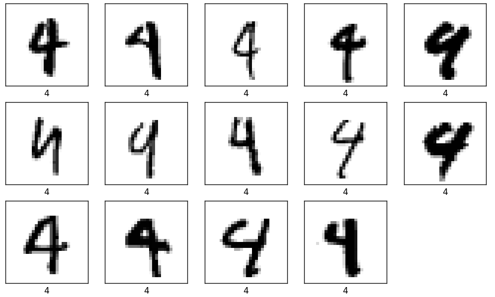
# number1을 number2로 예측한 경우
plt.figure(figsize=(10,10))
for i in range(len(number1_number2)):
plt.subplot(5,5,i+1)
plt.xticks([])
plt.yticks([])
plt.imshow(x[number1_number2[i]].reshape(28,28), cmap=plt.cm.binary)
plt.xlabel(t[number1_number2[i]])
plt.show()
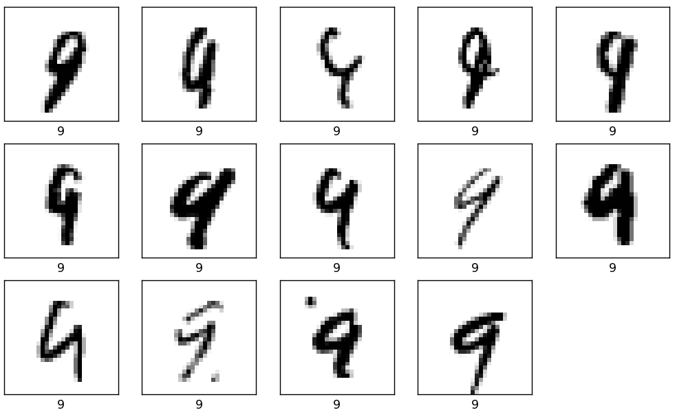
# number2을 number1로 예측한 경우
plt.figure(figsize=(10,10))
for i in range(len(number2_number1)):
plt.subplot(5,5,i+1)
plt.xticks([])
plt.yticks([])
plt.imshow(x[number2_number1[i]].reshape(28,28), cmap=plt.cm.binary)
plt.xlabel(t[number2_number1[i]])
plt.show()
# -------------------
# Confusion Matrix
[[ 967 0 0 1 1 3 2 1 3 2]
[ 0 1120 3 1 0 1 4 1 5 0]
[ 4 5 994 3 4 0 3 10 9 0]
[ 0 0 4 981 1 3 0 8 11 2]
[ 0 0 3 0 956 0 5 3 1 14]
[ 3 1 0 10 0 858 8 1 9 2]
[ 6 3 1 1 3 3 932 2 7 0]
[ 0 9 6 4 1 0 0 996 3 9]
[ 4 1 2 5 3 2 5 6 945 1]
[ 3 6 1 6 14 1 1 5 5 967]]
# -------------------
# accuracy Value
0.9716
# -------------------