[DL] CIFAR-10

🙋‍♂️ CIFAR-10 구성

CIFAR-10 Data Set은 32 x 32 크기의 60,000개의 Image Set으로 구성 되어 있으며,

10개의 Class로 분류 된다.각 Class는 60,000개의 전체 이미지와 50,000개의 Train Image, 10,000개의 Test Image로 구성

(Labels는 동일)

→ Mnist보다 가볍고, 시간이 덜 소요됨

 

✍ Data Set Load / Labels 확인

# Default import
import numpy as np # linear algebra
import pandas as pd # data processing, CSV file I/O (e.g. pd.read_csv)

import os

from tensorflow.keras.datasets import cifar10

# 전체 6만개 데이터 중, 5만개는 학습 데이터용, 1만개는 테스트 데이터용으로 분리
(train_images, train_labels), (test_images, test_labels) = cifar10.load_data()
print("train dataset shape:", train_images.shape, train_labels.shape)
print("test dataset shape:", test_images.shape, test_labels.shape)

# labels 확인
NAMES = np.array(['airplane', 'automobile', 'bird', 'cat', 'deer', 'dog', 'frog', 'horse', 'ship', 'truck'])
print(train_labels[:10])

# result
[6. 9. 9. 4. 1. 1. 2. 7. 8. 3.]

 

✍ Data Set / Preprocessing

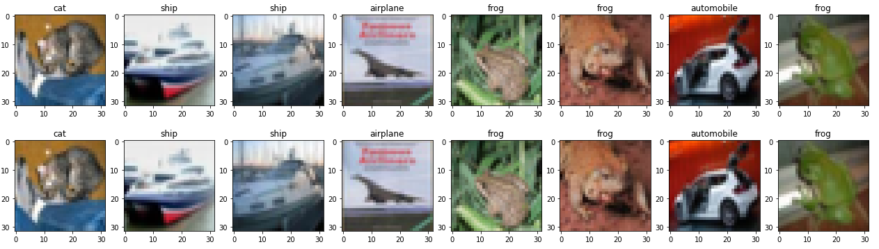
# Image Set 시각화

import matplotlib.pyplot as plt
import cv2
%matplotlib inline 

def show_images(images, labels, ncols=8):
    figure, axs = plt.subplots(figsize=(22, 6), nrows=1, ncols=ncols)
    for i in range(ncols):
        axs[i].imshow(images[i])
        label = labels[i].squeeze()
        axs[i].set_title(NAMES[int(label)])
        
show_images(train_images[:8], train_labels[:8], ncols=8)
show_images(train_images[8:16], train_labels[8:16], ncols=8)

# Image Set / Preprocessing
# image array의 0~255 사이의 값을 → /255하여 0 ~ 1 사이로 변환
(train_images, train_labels), (test_images, test_labels) = cifar10.load_data()

# test용으로 OHE 적용 안함, 여기서는 sparse categorical crossentropy 테스트를 위해 적용하지 않음. 
def get_preprocessed_data(images, labels):
    
    # 학습과 테스트 이미지 array를 0~1 사이값으로 scale 및 float32 형 변형. 
    images = np.array(images/255.0, dtype=np.float32)
    labels = np.array(labels, dtype=np.float32)
    
    return images, labels

# train, test에도 전처리 적용
train_images, train_labels = get_preprocessed_data(train_images, train_labels)
test_images, test_labels = get_preprocessed_data(test_images, test_labels)

 

✍ CIFAR10 Customizing / Layer 생성

from tensorflow.keras.models import Sequential, Model
from tensorflow.keras.layers import Input, Dense , Conv2D , Dropout , Flatten , Activation, MaxPooling2D , GlobalAveragePooling2D
from tensorflow.keras.optimizers import Adam , RMSprop 
from tensorflow.keras.layers import BatchNormalization
from tensorflow.keras.callbacks import ReduceLROnPlateau , EarlyStopping , ModelCheckpoint , LearningRateScheduler

IMAGE_SIZE = 32

input_tensor = Input(shape=(IMAGE_SIZE, IMAGE_SIZE, 3))

#x = Conv2D(filters=32, kernel_size=(5, 5), padding='valid', activation='relu')(input_tensor)
x = Conv2D(filters=32, kernel_size=(3, 3), padding='same', activation='relu')(input_tensor)
x = Conv2D(filters=32, kernel_size=(3, 3), padding='same', activation='relu')(x)
x = MaxPooling2D(pool_size=(2, 2))(x)

x = Conv2D(filters=64, kernel_size=(3, 3), padding='same', activation='relu')(x)
x = Conv2D(filters=64, kernel_size=(3, 3), padding='same')(x)
x = Activation('relu')(x)
x = MaxPooling2D(pool_size=2)(x)

x = Conv2D(filters=128, kernel_size=(3,3), padding='same', activation='relu')(x)
x = Conv2D(filters=128, kernel_size=(3,3), padding='same', activation='relu')(x)
x = MaxPooling2D(pool_size=2)(x)

# cifar10의 클래스가 10개 이므로 마지막 classification의 Dense layer units갯수는 10
x = Flatten(name='flatten')(x)
x = Dropout(rate=0.5)(x)
x = Dense(300, activation='relu', name='fc1')(x)
x = Dropout(rate=0.3)(x)
output = Dense(10, activation='softmax', name='output')(x)

model = Model(inputs=input_tensor, outputs=output)

model.summary()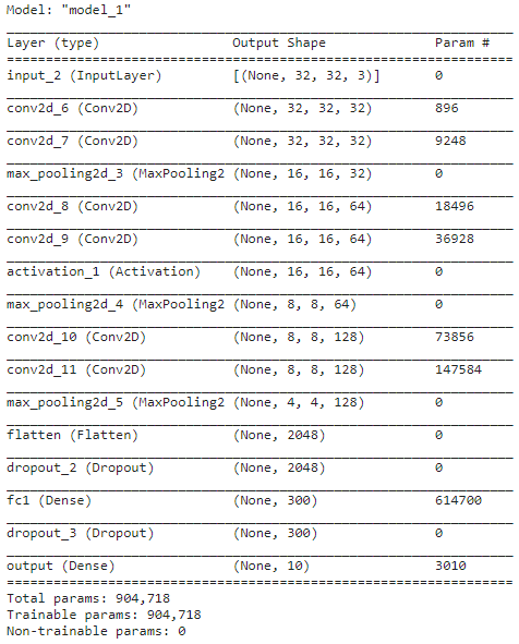

 

✍ CIFAR10 Customizing / Model 학습 수행 및 Test Data 검증

history = model.fit(x=train_images, y=train_labels, batch_size=64, epochs=30, validation_split=0.15) #7,500건을 validation에서 사용

# 일부 
2022-03-22 13:52:32.302979: I tensorflow/stream_executor/cuda/cuda_dnn.cc:369] Loaded cuDNN version 8005
665/665 [==============================] - 11s 7ms/step - loss: 1.6712 - accuracy: 0.3745 - val_loss: 1.4978 - val_accuracy: 0.4800
# 

import matplotlib.pyplot as plt
%matplotlib inline

def show_history(history):
    plt.figure(figsize=(6, 6))
    plt.yticks(np.arange(0, 1, 0.05))
    plt.plot(history.history['accuracy'], label='train')
    plt.plot(history.history['val_accuracy'], label='valid')
    plt.legend()
    
show_history(history)

# 테스트 데이터로 성능 평가
model.evaluate(test_images, test_labels)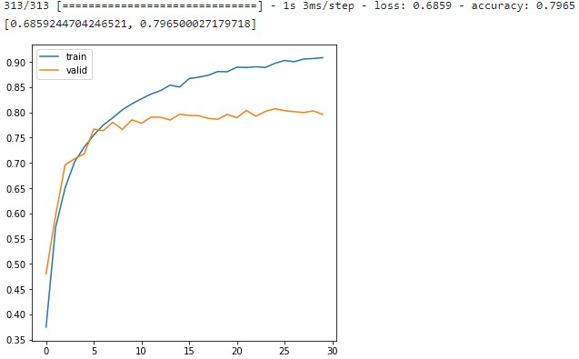

 

✍ CIFAR10 Customizing / model.predit()를 통한 이미지 분류 예측

# 테스트용 4차원 이미지 배열을 입력해서 predict()수행. 
# predict()의 결과는 softmax 적용 결과임. 학습 데이터의 원-핫 인코딩 적용 여부와 관계없이 softmax 적용 결과는 무조건 2차원 임에 유의 
preds = model.predict(np.expand_dims(test_images[0], axis=0))

print('예측 결과 shape:', preds.shape)
print('예측 결과:', preds)


predicted_class = np.argmax(preds, axis=1)
print('예측 클래스 값:', predicted_class)
# result ///
예측 클래스 값: [3 8 8 0 6 6 1 6 3 1 0 9 5 7 9 8 5 7 8 6 7 2 4 9 4 3 4 0 9 6 6 5]
# result ///


# image 출력
show_images(test_images[:8], predicted_class[:8], ncols=8)
show_images(test_images[:8], test_labels[:8], ncols=8)